

Knot Diagram Image Processing with OpenCV
- Jonathan

- Jun 28, 2023
- 9 min read
Updated: Jul 1, 2023
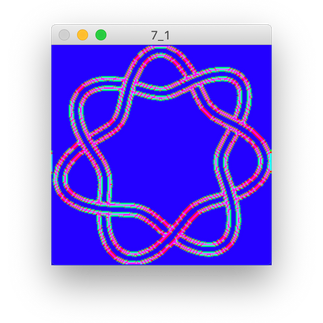
Recently, I've been playing around with OpenCV in Python, a package that gives us the ability to work with images and their pixels easily. My interest of course went to Knot Theory, so the pictures we'll be working with are Knot Diagrams! Doing so will give us cool pictures like

Can you tell what pattern we looked for to color this knot? If not, I'll talk about it at the end!
To start, a knot diagram is a 2D picture that represents a 3D knot by showing us a projection of the knot and making its crossings explicit. Here are a few examples:
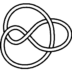
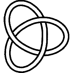
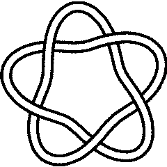
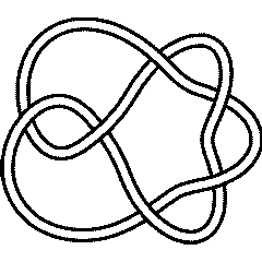
You can find these on the Knot Atlas. Or I'll save you some time and here is a folder containing all knot diagrams (in .gif and .png) up to 8 crossings.
I think these will be fun pictures to learn OpenCV with, so let's start.
Image Processing with OpenCV
The first thing to do is install OpenCV, which turns out to be surprisingly difficult. At least it was for me. The simple thing that should work is going to the Terminal and typing
pip install opencv-pythonThat failed for me, however, so I had to upgrade "pip":
pip install --upgrade pipBut it still failed! Specifically, the error was "failure to build wheels". What fixed this was upgrading both "setuptools" and "wheel".
pip install --upgrade setuptools wheelOnce we have that, we can start up our Python code and import OpenCV. The command to do this is "import cv2". We also want to import NumPy because our images will be stored as numpy arrays.
The first command to learn is "cv2.imread(path,flag)". It takes a path to an image and a flag for how to store the colors of each pixel. By default, it is stored as BGR (Blue, Green, Red). We can change that by entering any of these flags. For our diagrams, we'll tell OpenCV to read it in grayscale by using the flag "cv2.IMREAD_GRAYSCALE".
Since we have the Diagrams folder in the same spot as the .py file, we can use the os module's function "os.getcwd()" to get the current working directory (meaning the folder that the .py file is in), and then add the relative path "/Diagrams/KnotIndex.png" to load the image of whatever knot diagram we want. We call this by the Knot Index, which is of the form c_i, where c is the number of crossings and i is the index if we have multiple knots with that number of crossings.
For example, we have a single knot on 0, 3, and 4 crossings, which have knot index 0_1, 3_1, 4_1. Then there are two knots with 5 crossings, 5_1 and 5_2. We'll define this as a function called "KnotProcessing".
import cv2
import numpy as np
import os

def KnotProcessing(KnotIndex):
     PATH = os.getcwd()+f'/Diagrams/{KnotIndex}.png'
     img = cv2.imread(PATH, cv2.IMREAD_GRAYSCALE)
The next thing we want to do is actually see the picture. To do this, we use "cv2.imshow(caption,image)". The first entry will be the caption of the screen and the second is the image we want to show. For us, we'll just set the caption to the Knot Index. After that, we'll add "cv2.waitKey(0)", which means the program will wait until we hit any key. Then we add "cv2.destroyAllWindows()" so that when we do hit a key, we close the window.
import cv2
import numpy as np
import os

def KnotProcessing(KnotIndex):
     PATH = os.getcwd()+f'/Diagrams/{KnotIndex}.png'
     img = cv2.imread(PATH, cv2.IMREAD_GRAYSCALE)

     cv2.imshow(KnotIndex,img)
     cv2.waitKey(0)
     cv2.destroyAllWindows()
Here's what we see when calling "KnotProcessing('6_3')" and "KnotProcessing('7_1')".


For some reason, the backgrounds are different. So we'll do a loop through the image to "clarify" it, meaning if the pixel is dark enough, we set it to be black, and otherwise, we set it to be white. To get the dimensions, we use the NumPy array attribute ".shape", which will return the number of rows and columns our image has. Then we use the usual notation for getting entries of a NumPy array to get the pixel color value at that coordinate. So we add this code after we first read the image:
#clarify knot
r,c = img.shape
for i in range(r):
     for j in range(c):
          if img[i,j] < 20:
               img[i,j] = 0
          else:
               img[i,j] = 255
And our new outputs look like this:


This function will be our template for all the image processing we decide to do. Whatever we decide, we'll define a function describing that process outside "KnotProcessing" and then just pass it in. This will make the code look much nicer and less cluttered.
def KnotProcessing(KnotIndex):
     PATH = os.getcwd()+f'/Diagrams/{KnotIndex}.png'
     img = cv2.imread(PATH, cv2.IMREAD_GRAYSCALE)
     #clarify knot
     r,c = img.shape
     for i in range(r):
          for j in range(c):
               if img[i,j] < 20:
                    img[i,j] = 0
               else:
                    img[i,j] = 255

     #processing
     img = ProcessFunction(img)

     #display
     cv2.imshow(KnotIndex,img)
     cv2.waitKey(0)
     cv2.destroyAllWindows()
Now all we have to do is switch out the ProcessFunction!
Coloring our Knot Diagrams
Now that our image is set up, there are lots of different things we could choose to do, but let's start simple. A lot of these functions will be based on the neighbors of the given pixel, which we can get using array slicing. This is amazing, by the way, because what I did first was write out almost 15 lines of "if-else" statements to account for edges and corners. But with array slicing and min/max operators, we get the correct neighbors in one line!
def get_neighbors(pixel,image):
     r,c = image.shape
     image[pixel[0],pixel[1]] = 1
     return image[max(pixel[0] - 1,0):min(pixel[0]+2,r), max(pixel[1] - 1,0): min(pixel[1] + 2,c)]
We add the line "image[pixel[0],pixel[1]] = 1" to distinguish the pixel we start with, since it's unclear when we're working with an edge or corner pixel. I'll call such a pixel the root of the neighborhood. Let's test this within our KnotProcessing function, using the trefoil, 3_1.
#processing
img1 = get_neighbors((30,100),img)
img2 = get_neighbors((0,0),img)
img3 = get_neighbors((0,50),img)
img4 = get_neighbors((r-1,c-1),img)
print(img1) #output:
[[  0   0   0]
 [  0   1   0]
 [255   0   0]]
print(img2) #output:
[[1 255]
 [255 255]]
print(img3) #output:
[[255 1 255]
 [255 255 255]]
print(img4) #output:
[[255 255]
 [255   1]]
One of the things we can use this for is to blur our image! We first create a reference image, get the shape, then start looping through pixels. For each pixel, we get the neighbors, get the shape of the neighbor array, and loop through all non-root pixels, adding their value to a variable called darkness. At the end, we divide by the number of pixels we looked at. So our blurring function is replacing a pixels value with the average value of its neighbors.
def blur(image):
     ref_img = image
     r,c = image.shape
     for i in range(r):
          for j in range(c):
               N = get_neighbors((i,j),ref_img)
               Nr, Nc = N.shape
               darkness = 0
               for a in range(Nr):
                    for b in range(Nc):
                         if N[a,b] != 1:
                              darkness += N[a,b]
               darkness /= (Nr*Nc - 1)
               image[i,j] = int(darkness)
     return image
Here is the output! First the original, then blurred once, twice, and finally blurred 10 times. We accomplish these repeated blurrings with a loop "for _ in range(10): img = blur(img)"


That works well! Let's define a new function that colors a pixel based on how many of its neighbors are black pixels. If we just look at the four cardinal directions, we get pictures like


But let's do all 8 neighbors and choose our color palette with a bit more thought. This website gives us a palette (I believe via machine learning!) of visually distinct colors. The 9 colors we'll use (in RGB) are:
colors = [(0,100,0), (188,143,143), (255,0,0),
          (255,215,0), (0,255,0), (65,105,225),
          (0,255,255), (0,0,255), (255,20,147)]
We'll call the function "color_by_count" and it looks very similar to "blur". One big difference is that we need add a color conversion (from GRAYSCALE to BGR and from BGR to RGB) using "cv2.cvtColor(image,flag)". All together, this makes
def color_by_count(image):
     ref_img = image
     r,c = image.shape
     image = cv2.cvtColor(image,cv2.COLOR_GRAY2BGR)
     colors = [(65,105,225), (188,143,143), (255,20,147),
               (255,0,0),(255,215,0), (0,255,0),
               (0,255,255), (0,100,0), (0,0,255)]
     for i in range(r):
          for j in range(c):
               N = get_neighbors((i,j),ref_img)
               Nr, Nc = N.shape
               count = 0
               for a in range(Nr):
                    for b in range(Nc):
                         if N[a,b] == 0:
                              count += 1
               image[i,j] = colors[count]
     image = cv2.cvtColor(image,cv2.COLOR_BGR2RGB)
     return image
Shuffling around the colors list gives us a bunch of funky versions of our knot diagrams:


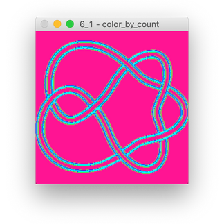

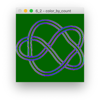
Especially with the two on the right, we see a small pattern that hopefully we can make more exact for later uses - the coloring looks like it's kind of highlighting the crossings! This would make sense, because the areas with crossings have a lot of black pixels. But it also picks up on the more bendy strands of the knot, which we wouldn't want.
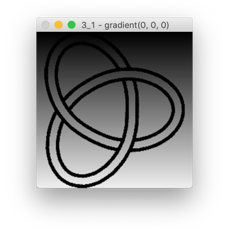
Anyway, let's make another function! This one we'll call "gradient" because we'll add a color gradient to the background of the knot. It will take in an image and a starting color and the gradient will get lighter as we go down the rows. We form the colors from the gradient like so:
gradient_colors = [(min(color[0] + i,255),
                    min(color[1] + i,255),
                    min(color[2] + i,255)) for i in range(r)]
With OpenCV, this really isn't hard! We just sort through the pixels like in the other function, checking the reference image for whether that pixel is black, and if not, we set it equal to "gradient_colors[i]" if it is in row "i". Here's what we have:
def gradient(image,color):
     ref_img = image
     r,c = image.shape
     image = cv2.cvtColor(image,cv2.COLOR_GRAY2BGR)
     gradient_colors = [(min(color[0] + i,255), min(color[1] + i,255), min(color[2] + i,255)) for i in range(r)]
     for i in range(r):
          for j in range(c):
               if ref_img[i,j] != 0:
                    image[i,j] = gradient_colors[i]
     image = cv2.cvtColor(image,cv2.COLOR_BGR2RGB)
     return image
Let's test this with a few different colors and knots:


Let's go ahead and add the functionality to turn the gradient. We'll add a parameter "direction" that defaults to "down", but takes in "up", "right", "down", "left", "diagonal", and "doublediagonal". Then within our double for loop through the pixels, we'll add this:
if ref_img[i,j] != 0:
     if direction == 'down':
          image[i,j] = gradient_colors[i]
     elif direction == 'up':
          image[i,j] = gradient_colors[-i]
     elif direction == 'right':
          image[i,j] = gradient_colors[j]
     elif direction == 'left':
          image[i,j] = gradient_colors[-j]
     elif direction == 'diagonal':
          image[i,j] = gradient_colors[
          min((i + j)//2,len(gradient_colors) - 1)]
     elif direction == 'doublediagonal':
          image[i,j] = gradient_colors[
          min(max(-i + j, i - j),len(gradient_colors) - 1)]
     else:
          image[i,j] = gradient_colors[i] #down
Sticking with knot 6_2 and switching the colors around, here are a few examples:


Coloring by Knot Segments
Ok, let's get that original picture that we put up at the very beginning! This is by far the most mathematical function we've defined so far. We go through each column and draw a downward ray, counting the number of strands we pass through. Then we color the entire segment of that strand based off that count! So if it's the first strand we encounter, we color it blue. The next, red, then green, and so on.
To be clear, I'm considering a strand to be a continuous sequence of black pixels. Since we're just casting a downward ray, it simplifies things. We define "col_segments(ind, b_set)" to take in a column index "ind" and a list "b_set" that we want to sort (the b stands for boundary). We start by initializing an empty list of segments, the column, and the current segment. If the column is empty, we return the empty list, meaning no segments.
def col_segments(ind,b_set):
    segments = []
    col = [b for b in b_set if b[1] == ind]
    segment = []
    if len(col) == 0:
        return []
Next, we go through each pixel of the column, adding it to "segment". We add a check to return "segments" if we've reached the end of the column. Otherwise, we check to see if two elements of "col" are directly next to each other or not with "elif col[i+1][0] - col[i][0] > 2". If that happens, we've reached the end of a segment, so we add that segment to "segments" and then reinitialize "segment = []".
Though we do run into an issue if the very last pixel is a part of the previous segment, so we'll add a special line for that case. Then as we loop, it'll do the whole process! Once the loop is done, we return "segments".
     else:
          for i in range(len(col)):
               segment.append(col[i])
               if i == len(col)-1:
                    segments.append(segment)
                    break
               elif col[i+1][0] - col[i][0] > 2:
                    segments.append(segment)
                    segment = []

     return segments
Instead of seeing lists, let's go ahead and implement this as a knot coloring function to see some example! Then we define "color_by_col_segments", which starts similarly to the previous functions, except we define the "boundary" to be all pixels that are black in the Knot Diagram.
def color_by_col_segments(image):
     ref_img = image
     r,c = image.shape
     colors = [(0,0,255),(255,0,0),(0,255,0),(255,255,0),(255,0,255),(0,255,255),(0,128,255),(128,0,255),(255,128,0),(255,0,128),(0,255,128),(128,255,0),(128,255,128),(128,128,255)]
     boundary = [(i,j) for i in range(r) for j in range(c) if ref_img[i,j] == 0]
We convert our image to color, and then loop through each column, getting that column segment list. Then we loop through that list, getting a segment, and coloring each pixel in that segment a color based on the segment number. Finally, we return our image.
     image = cv2.cvtColor(image,cv2.COLOR_GRAY2BGR)
     for i in range(c):
          col_segs = col_segments(i,boundary)
          for j in range(len(col_segs)):
               segment = col_segs[j]
               for pixel in segment:
                    image[pixel[0],pixel[1]] = colors[j]
     image = cv2.cvtColor(image,cv2.COLOR_BGR2RGB)
     return image
The double color conversion is weird, but for some reason, having "cv2.COLOR_GRAY2RGB" only at the top still converts it to BGR. So we just convert it to that in the first place to color the pixels, then we convert it to RGB at the end. I love the pictures this makes!


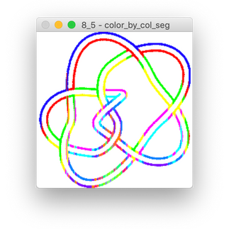
Casting the downward ray from different columns will give similar but not exactly the same results as the previous column, which is why the knots have an almost "dripping paint" kind of style. And finally, if we look at knot 5_1, we get the first image in the post!

Now what if we wanted to add two of these effects at once? We can't just pass one processed image into the the next function because it isn't in grayscale. So instead, we create two separate images and then merge them. Here's how this looks within the whole "KnotProcessing" function.
def KnotProcessing(KnotIndex):
     PATH = os.getcwd()+f'/Diagrams/{KnotIndex}.png'
     img = cv2.imread(PATH, cv2.IMREAD_GRAYSCALE)
     #clarify knot
     r,c = img.shape
     for i in range(r):
          for j in range(c):
               if img[i,j] < 20:
                    img[i,j] = 0
               else:
                    img[i,j] = 255

     #processing
     ref_img = img
     img1 = color_by_col_segments(img)
     img2 = gradient(img,(20,0,50),'doublediagonal')
     img = cv2.cvtColor(img,cv2.COLOR_GRAY2RGB)
     for i in range(r):
          for j in range(c):
               if ref_img[i,j] == 0:
                    img[i,j] = img1[i,j]
               elif ref_img[i,j] == 255:
                    img[i,j] = img2[i,j]

     #display
     cv2.imshow(KnotIndex+f' - col_seg + gradient',img)
     cv2.waitKey(0)
     cv2.destroyAllWindows()
And they look great!


Thank you for reading!
Jonathan M Gerhard


Comments