Image Processing Algorithms with OpenCV

We'll start with the same general layout for an image processing function as last post.

import os
import cv2
import numpy as np

def ImageProcessing(image):
     #get image
     PATH = os.getcwd()+f'/{image}'
     img = cv2.imread(PATH)

     #processing
     img = ProcessFunction(img)

     #display
     image_name = image.strip('.jpg')
     cv2.imshow(image_name,img)
     cv2.waitKey(0)
     cv2.destroyAllWindows()

We get the "current working directory" to where our .py file is (which is also where your image needs to be), add a "/" and the image name to it, and then use "cv2.read" to load the image as a NumPy array. We'll define whatever processing we want outside this function and replace "ProcessFunction" with that function. Finally we display the image using "cv2.show", getting the window name by stripping the entered image name of its extension (in this case, ".jpg"). Finally, we tell OpenCV to close the window when any key is pressed.

Now I want to try to focus on some processing functions that are a bit more picture-oriented rather than knot--diagram-specific. Don't get me wrong, OpenCV has a massive library of image processing functions, but there are plenty of good posts on that, so I want to instead just try to define some of our own.

First, we'll copy over the "get_neighbors" function we defined last time, with a small change. We add a parameter "size", which tells us the size of the square neighborhood we want.

def get_neighbors(pixel,image,size):
     r,c = image.shape
     image[pixel[0],pixel[1]] = 1
     return image[max(pixel[0] - size,0):min(pixel[0]+size+1,r), max(pixel[1] - size,0): min(pixel[1] + size+1,c)]

The picture I'll be using will be of my adorable cat, Lady!

And the first function I want to define is the "pixelate" function. We'll take in an image and desired pixel size and make a copy as a reference image. We get the number of rows and columns and use "_" for the third value of "image.shape", which will be 3 since we're using BGR, the default for OpenCV. We use "_" because we'll never reference that number again, but still need to unpack it.

def pixelate(image,pixel_size):
     ref_img = image
     r,c, _ = image.shape
     for i in range(0,r,pixel_size):
          for j in range(0,c,pixel_size):
               #color box
               center = ref_img[min(i + pixel_size//2,r-1), min(j + pixel_size//2,c-1)]
               for a in range(pixel_size):
                    for b in range(pixel_size):
                         if i + a < r and j + b < c:
                              image[i+a,j+b] = center
     return image

Now, we could use "cv2.resize" to literally shrink the image, but I want to keep the dimensions the same and just view it as pixel art. Which means we'll loop over "i" and "j" taking the step size to be "pixel_size". Then inside that, we'll record the color of the center pixel and go through another loop through that square, coloring every pixel the color of the center.

Let's see what this does to my cat! We'll run one with pixel size 30, one with pixel size 60, and the last with pixel size 300. Can you still see her in that last picture?

If we look at any pixel in BGR, we could define its darkness to be B+G+R. The smaller it is, the darker the pixel is. Let's define a "darkness_cutoff(image,cutoff)" function that scans through "image" and checks if a pixel has a darkness less than "cutoff", an integer. If so, it sets it black, and otherwise we set it white. We'll use type hints for clarity here.

def darkness_cutoff(image,cutoff: int):
     r,c,_ = image.shape
     for i in range(r):
          for j in range(c):
               if sum(image[i,j]) < cutoff:
                    image[i,j] = [0,0,0]
               else:
                    image[i,j] = [255,255,255]
     return image

and here's the output with darkness cutoff 100, 200, 300, and 400.

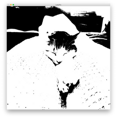
We could also do a cutoff for all values being less than a given pixel. We'll again use type hints to make it clear that in this case, cutoff should be a list. The code is exactly the same as above except the "if" statement is swapped out with "if (image[i,j] < cutoff).all():" to check if all three entries are less than the corresponding entries of cutoff. If so, we do nothing, but if something fails the cutoff, we'll set it to be a white pixel. Here are cutoffs

[100,100,100], [0,50,100], [200,100,200], [20,100,256]

Notice the second image is all white because no image can have its first value less than 0. So another interesting thing we could do with the pixel cutoff is looking at values like

[256,10,10], [10,256,10], [10,10,256]

This is essentially isolating the Blue, Green, and Red channels of the image.

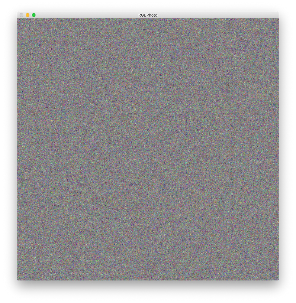
The effect is much clearer with a more colorful image: this beautiful image by Alexander Grey.

Full disclosure, the green did require upping the cutoff to [60,256,60] to see it better.

But OpenCV Images are NumPy Arrays, Right?

Indeed they are! So why don't we start treating them as such? We have a ton of different matrix operations we could do to the image if we treat it as a matrix itself. The simplest thing we can do is add two matrices together and for example, if we wanted to brighten or darken an image, this amounts to adding or subtracting "(1,1,1)" from each pixel. We could accomplish this with a bunch of loops, but NumPy has a built-in "add" function that adds two NumPy arrays element-wise!

And it has a built-in function for creating an array of a certain shape filled with given value. We can get our array full of "(1,1,1)"s by writing

B = np.full((r,c,3),(1,1,1),dtype = np.uint8)

That last part "dtype = np.uint8" is very important. NumPy arrays default to Data Type "int64", but OpenCV expects Data Type "uint8". If you run the program and just get a black screen, then you forgot this line!

Then we use "np.add(image,B)" to brighten the image by 1. We'll run this 100 times on LadyPic and see what we get:

Whoa! Do you see what went wrong? We had values above 255! And OpenCV just loops those values mod 256 to fix that when showing the image. Honestly, it looks cool enough that I'm going to copy it over to its own function "brighten_unbound" so we can play with it more later. We'll define a similar "darken_unbound" by using "np.subtract(image,B)" instead of np.add. Here is what it looks like to apply this 100 times to LadyPic.

Really cool! But let's do it correctly now for the "brighten" function. If we go over 255 in any spot, we need to set it to 255. There are certainly ways to do this with NumPy ("np.full", "np.add", and "np.where") but I'm just going to do a loop because it's simpler. Here it is:

def brighten(image,I):
     r,c,_ = image.shape
     for i in range(r):
          for j in range(c):
               image[i,j] = [min(255,image[i,j][0]+I),
               min(255,image[i,j][1]+I),min(255,image[i,j][2]+I)]
     return image

Let's see it working with intensity I = 50,100,150,200.

We can define a "darken" function in the exact same way with "min(255,image[i,j][1]+I)" replaced with "max(0,image[i,j][1] - I)". Here is I = 50,100,150.

Another thing we could do is actually add two images together! This will of course cause some overflow, but let's see what it looks like when we add the two images we've been working with together. First we need to resize the more colorful picture to be the same size as LadyPic, which I'll do in Krita. The following code will load the first image, show you it, wait till you click a key, then load and show the second image until you click a key, then show you the addition of the two images.

def add_images(image1,image2):
     #get images
     PATH1 = os.getcwd()+f'/{image1}'
     img1 = cv2.imread(PATH1)
     img1_name = image1.strip('.jpg')
     cv2.imshow(img1_name,img1)
     cv2.waitKey(0)
     PATH2 = os.getcwd()+f'/{image2}'
     img2 = cv2.imread(PATH2)
     img2_name = image2.strip('.jpg')
     cv2.imshow(img2_name,img2)
     cv2.waitKey(0)

     #process
     img = img1+img2
     #display
     image_name = img1_name + img2_name
     cv2.imshow(image_name,img)
     cv2.waitKey(0)
     cv2.destroyAllWindows()

Let's see what we get!

That's cool - the two spikes in the center of BGRPhotoResized fit well with Lady's ears! If we darken the second image a bit, it'll contribute a little less to changing each pixel. Remember that an all black image would be the identity element here.

But this isn't blending them, really. Maybe we could try to average the pixels of the two images? Let's add a "how" parameter that defaults to the normal add, then add a few if statements down where we add the images.

#process
     r,c,_ = img1.shape
     if how == 'normal':
          img = img1+img2
     if how == 'average':
          new_image = img1
          for i in range(r):
               for j in range(c):
                    new_image[i,j] = (img1[i,j]+img2[i,j])//2
          img = new_image

But since we're just dividing by 2, this is really just doubling the darkness of the image. Let's try something where we keep the darkness the same as the first image but try to preserve the hue. We could try a few different things. The first is multiplicative scaling. For each pixel coordinate, we calculate both images' darkness at that spot and then scale the second pixel by the appropriate amount for it to have the correct darkness (or as close as possible).

if how == 'darkness_transfer_mul':
     new_image = img1
     for i in range(r):
          for j in range(c):
               px1 = img1[i,j]
               d1 = px1[0]//3 + px1[1]//3 + px1[2]//3
               px2 = img2[i,j]
               d2 = px2[0]//3 + px2[1]//3 + px2[2]//3
               if d2 != 0:
                    scaling_factor = d1/d2
                    new_px = [min(255,round(scaling_factor*px2[0])),min(255,round(scaling_factor*px2[1])),min(255,round(scaling_factor*px2[2]))]
               else:
                    new_px = img2[i,j]
               new_image[i,j] = new_px
     img = new_image

Here is "add_images('LadyPic.jpg','BGRPhotoResized.jpg','darkness_transfer_mul')".

And here is "add_images('BGRPhotoResized.jpg','LadyPic.jpg','darkness_transfer_mul')".

Wow, the way Lady and the fairly plain background is swirled by the textured image by Alexander Grey in the second image is wonderful! And how colorful we were able to make Lady in the first picture is great too. They both look much cooler than the simple additions.

Let's now do the same thing but with an additive scaling. So we calculate the difference "d1 - d2" of darkness of the two pixels and then add a third of that value to each coordinate of the second image (or as close as possible). We'll need to have a few "if" statements for whether the difference is positive (so we use "min(255,blah)") or negative ("max(0,blah)"). Here's that:

if how == 'darkness_transfer_add':
          new_image = img1
          for i in range(r):
               for j in range(c):
                    px1 = img1[i,j]
                    d1 = px1[0]//3 + px1[1]//3 + px1[2]//3
                    px2 = img2[i,j]
                    d2 = px2[0]//3 + px2[1]//3 + px2[2]//3
                    scaling_factor = d1 - d2
                    if scaling_factor > 0:
                         new_px = [min(255,px2[0] + scaling_factor//3),min(255,px2[1]+ scaling_factor//3),min(255,px2[2]+ scaling_factor//3)]
                    elif scaling_factor < 0:
                         new_px = [max(0,px2[0] + scaling_factor//3),max(0,px2[1]+ scaling_factor//3),max(0,px2[2]+ scaling_factor//3)]
                    else:
                         new_px = img2[i,j]
                    new_image[i,j] = new_px
          img = new_image

And here it is with "LadyPic + BGRPhotoResized" on the left and "BGRPhotoResized + LadyPic" on the right.

So we see the additive scaling causes a much smaller change in the original image. But look very closely at that first image and you'll see Lady appear! It's almost like she's hiding under all the painted swirls.

We can also bring some real math into this. We can define the darkness of a (B,G,R) value to be B + G + R (or dividing by 3 if needed because of overflow in Python). We can also define the hue mathematically: We find the maximum color value, the minimum color value, and then use one of three formulas:

• If B = max, then hue = 4 + (R-G)/(max-min)

• If G = max, then hue = 2 + (B-R)/(max-min)

• If R = max, then hue = (G-B)/(max-min)

So to check our above operations (without thinking of the min/max stuff inside for simplicity), we clearly transfer the darkness, but how successful are we at preserving hue? For multiplicative scaling by sf, our pixel goes from

(B,G,R) --> (B*sf, G*sf, R*sf)

so sf is a factor in all B,G,R,max,min, which means they cancel out and hue is unchanged!

For the additive scaling, we go from

(B,G,R) --> (B + sf, G + sf, R + sf)

which means the maximum and minimum stay the same. It also means that any B - R, R - G, or

G - B will have sf cancel out. So it remains unchanged! In reality, the min/max we had to do to keep the pixels between 0 and 255 will change the hue and darkness slightly, but it's good to know that in theory, we've done what we want.

If we remove that correction and allow it to overflow, we will perfectly maintain hue and perfectly transfer darkness...mod 256. Let's see what this looks like by defining "unbound" versions of "darkness_transfer_mul" and "darkness_transfer_add".

Here are bound/unbound versions of "darkness_transfer_mul" for LadyPic+BGRPhotoResized.

And for BGRPhotoResized+LadyPic.

You can see in both examples the overflow artifacts in the unbound images. For the first there is a lot more blue spotting and for the second we get a lot of small green specks. Now let's do "darkness_transfer_add". Here are bound/unbound versions of LadyPic+BGRPhotoResized.

And bound/unbound versions of BGRPhotoResized+LadyPic.

I'm not sure if I see any difference for the second image, but look at the first one! A lot of overflow in the upper portion. But you can still see Lady's face peaking through the middle.

Another thing we can do with matrices is take products. The Hadamard Product is a multiplication of matrices that multiplies element-wise. With NumPy, we call "np.multiply(A,B)" to get the Hadamard Product of "A" and "B". Here is a simple function to calculate repeated Hadamard products of a matrix with itself:

def hadamard_power(image,n):
     for _ in range(n):
          image = np.multiply(image,image)
     return image

Let's see what it looks like for n = 0 up to 5.

That's very cool! It somewhat maintains the shape of the image but the colors are very distorted and as we repeat multiplications, the image gets blurred.

Now I want to do usual matrix multiplication. But we don't have matrices, we technically have a tensor of shape (r,c,3), so how do we multiply these? There are various tensor products (in NumPy, we'd use "np.tensordot"), but I'm going to define our own product to be sure that we end up with an array of the correct shape, (r,c,3).

How I'll do this is to take our image and split it into its three separate channels, BGR. This is easy with array slicing. We put a ":" in the first two spots to say we want all those values, but then we pick the third value according to the channel. These images are grayscale, with the intensity representing how much that channel contributes to the pixel color.

def get_channels(image):
     Bimage = image[:,:,0]
     Gimage = image[:,:,1]
     Rimage = image[:,:,2]

     return Bimage,Gimage,Rimage

We'll use Alexander Grey's image again for a better example of the BGR channels.

Now that these are actual matrices, I'm going to take each matrix M and return M*M^T, where M^T is the transpose of M. This way, even if we have a non-square matrix, we can still do the product. Then finally, we recombine them. Here is the code:

def matrix_transpose_power(image,n):
     r,c,_ = image.shape
     Bimg, Gimg, Rimg = get_channels(image)
     Bimg2 = np.matmul(Bimg,np.transpose(Bimg))
     Gimg2 = np.matmul(Gimg,np.transpose(Gimg))
     Rimg2 = np.matmul(Rimg,np.transpose(Rimg))
     new_image = np.zeros((r,c,3))
     for i in range(r):
          for j in range(c):
               new_image[i,j] = [EnB[i,j],EnG[i,j],EnR[i,j]]
     return new_image

What does the result look like?

Unfortunately not much! Most other product-involved operations result in an image like this. But that's not necessarily a bad thing! If we scramble it like this but have a way to unscramble it, then we've just made a very basic version of encryption/decryption algorithms for images. I'll try to expand on that idea later. For now, I want to look at some recursive algorithms.

Recursive Algorithms for Image Processing

What I mean by "recursive algorithm" is a function that performs some action on a pixel based on its neighbors, then moves to the next pixel and performs the same action based on its neighbors, and so on. Since we're not using a reference image like before, the changes we make to one pixel will propogate to the others. This is an example of a cellular automaton. A very famous example of such a system is Conway's Game of Life. Though that does update every cell in the grid at once, so it's still slightly different.

The rule I want is for each pixel to distribute some of its color to its neighbors. Specifically, we'll send a bit of our blue upward, a bit of our green downward, and a bit of the red to the left and right. Even more specifically, that bit will be 50%. Like I feared for the "get_neighbors" function, this will be a bunch of "try-except" statements. Not the most efficient way to do this, surely, but it works for now!

def recursive_distribute(image,pixel):
     r,c, _ = image.shape
     Bp, Gp, Rp = image[pixel[0],pixel[1]]
     try:
          color = image[pixel[0] - 1, pixel[1]]
          image[pixel[0] - 1, pixel[1]] = [min(255,color[0] + Bp//2), color[1],color[2]]
          image[pixel[0],pixel[1]] = [max(0,Bp - Bp//2), Gp, Rp]
     except:
          ...
     try:
          color = image[pixel[0] + 1, pixel[1]]
          image[pixel[0] + 1, pixel[1]] = [color[0], min(255,color[1] + Gp//2),color[2]]
          image[pixel[0],pixel[1]] = [Bp, max(0,Gp - Gp//2), Rp]
     except:
          ...
     try:
          color = image[pixel[0], pixel[1] - 1]
          image[pixel[0], pixel[1] - 1] = [color[0], color[1],min(255,color[2] + Rp//4)]
          image[pixel[0],pixel[1]] = [Bp, Gp, max(0,Rp - Rp//4)]
     except:
          ...
     try:
          color = image[pixel[0], pixel[1] + 1]
          image[pixel[0], pixel[1] + 1] = [color[0], color[1],min(255,color[2] + Rp//4)]
          image[pixel[0],pixel[1]] = [Bp, Gp, max(0,Rp - Rp//4)]
     except:
          ...
     
     return image

Then we'll define another function "distribute" that loops through the pixels and applies this.

def distribute(image):
     r,c,_ = image.shape
     for i in range(r):
          if i%50 == 0:
               print(i)
          for j in range(c):
               image = recursive_distribute(image,(i,j))
     return image

I will say that this takes a pretty long amount of time! So I'm going to sketch up a smaller 240x240 image in Krita to apply this to. Here is the original image, then applying "distribute" 1, 2, 3, 4, and 5 times.

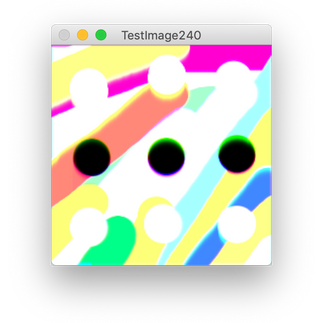
And if we apply it 30, 50, and 100 times, we get

Honestly, it's a bit strange! We have this upper-right purple part that stabilizes, a purple line up top, an aqua blue line along the right, but everything else gets washed out. I've run it 300 times and that's still the case. Let's do the same thing we've been doing and create an unbound version of this function where we don't apply "min(255,blah)" or "max(0,blah)" and allow the overflow.

This will certainly cause a difference. Our image being washed out with white means that we capped a lot of pixels at 255 to prevent overflow. The unbounded versions will not lose any color, but simply distribute it mod 256. Here are 12 images with unbounded distribute applied 0, 1, 2, 3, 4, 5, 30, 50, 100, 200, 300, and 400 times.

Quite a big difference! But what surprises me are the similarities that remain. The three middle blue ovals after 30 applications and the upper-right area that is mostly purple and unchanged. The three new images at 200, 300, and 400 applications show that even with overflow, there may be a stable state or loop.

I'll have to look into the algorithm and try to mathematically describe what's happening. I'll also explore some more well-established algorithms in the next post. But for now, I think this post is long enough!

Thank you for reading!

Jonathan M Gerhard