

Image Processing Algorithms with OpenCV 3
- Jonathan

- Jul 2, 2023
- 12 min read
In the last post, we wrote a "Palette-Simplifying" algorithm which took in a picture and a palette of colors, then redrew the picture as closely as possible using only colors in that palette. This produces images that look incredibly interesting depending on which palette you choose. But what I want to do now is turn this into a process that only takes in an image and a percentage. That percentage (between 0 and 1) will be the ratio of the number of colors we want our palette to have to the total number of distinct colors in the image.
Once we have this, we can apply "paletteSimplify" to repaint our image in a smaller amount of colors. We'll call this process "autoPaletteSimplify" because we form the palette from the image. We start in the usual way:
def autoPaletteSimplify(image,p):

    #get_image
    PATH = os.getcwd()+f'/{image}'
    img = cv2.imread(PATH)
    r,c,_ = img.shape

    #autoPS
    colorset = []
    palette = []

    #display
    paletteSimplify(image,palette)
We've also initiated our full colorset and our palette. We then loop through the pixels and add their color to "colorset". A very important step here, which we discussed a bunch last post, is that we convert the colors [B,G,R] into tuples (B,G,R) before adding them to color set. If we didn't, then we wouldn't be able to check list containment, because lists/nparrays are mutable while tuples are immutable.
for i in range(r):
          for j in range(c):
               color = tuple(img[i,j])
               if color not in colorset:
                    colorset.append(color)
Now that we have our full set of distinct colors, we want to choose a palette. We could do this (pseudo)randomly very easily. Use the random module method "random.random()" to generate a random float between 0 and 1. If this is less than the given percentage p, then add it to the palette. This would give the correct count, probabilistically. So we'll add a "how" keyword to our function and add the following code after generating "colorset":
#autoPS
...

if how = 'random':
    for color in colorset:
        r = random.random()
        if r < p:
            palette.append(color)
Let's see how this looks, with our Smeared240 image. The total number of colors in this image is 30374, and we'll set our percentage to "p = 0.01". Now we run the code
P = autoPaletteSimplify('Smeared240.png',0.01,'random')An error we quickly run into is an overflow error because our tuples have data type uint8, meaning they are unsigned 8-bit integers, i.e. from 0 to 255. Our distance we're calculating is way bigger than that, so we get an error. So inside the "bestMatch" function, we add a conversion of our pixel to 'int64' with "pixel = np.int64(pixel)" and then within the color loop, we add "color = np.int64(color)".
On the left is the original, and on the right is the autosimplified version with 337 colors.


We don't see too much difference except the simplified version doesn't have as smooth of transitions between colors. And here are a few examples with "p = 0.001".


Honestly, they all look better than I expected! To really demonstrate the issue with the random approach, here are a few examples with "p = 0.00003".


These look interesting in their own right, but if you're looking for a faithful recreation of your image with a simplified palette, this isn't it. By randomly choosing colors, we get a randomly colored picture. So let's add a "how = 'smart'" section, where we'll choose the colors of our palette a little more carefully. We'll start by figuring out how many distinct colors we have and multiplying that by our given percentage to see how many colors we need in the palette.
#SMART
if how == 'smart':
    AC = len(colorset)
    PC = int(AC*p)
Now here's the wonderful mathematical question:
How do we generate PC colors from our list of AC colors so that they are as evenly spaced out as possible?
Well, one of the very first algorithms one might learn is the greedy algorithm. It's a strategy for maximizing a value where you just take the best possible value at each step. This might seem like it would produce the best result, but it can actually produce fairly bad results. This is because we're making the best local decision at each step but not taking into account the global situation. In other contexts, this is called the Farthest-First Traversal, for clear reasons.
Another algorithm that gives a set of evenly spaced points is Lloyd's Algorithm. Or we have Fortune's Algorithm, which is responsible for the beautiful Voronoi Diagrams. In addition to the 2D version, there are a variety of amazing 3D models made up of Voronoi cells. And Blender even has a texture node for Voronoi mesh! Wikipedia has a wonderful animation of Voronoi cells being formed:

Building Voronoi Diagrams
With a variety of methods attributed to many people (Voronoi, Delaunay, Dirichlet,...), let's now implement the Voronoi cell creation here! There are a variety of sophisticated algorithms to do this, as I've already mentioned. But what we'll do is the "obvious" idea. Take an input set of starting points and assign each a color, then scroll through all the points in your surface and calculate their distance from each given point in the set. Then color it according to which point it's closest to.
So let's define a function "Voronoi(*dims,roots,colors)". The asterisk "*dims" allows us to enter an arbitrary number of dimensional arguments. So if we want a 2D Voronoi Diagram, we'd pass in a width and height. If we wanted it 3D, we'd add a third number, and so on. Then we have our keyword arguments "roots" and "colors". We'll check to make sure these are the same length, and return an error if not.
def Voronoi(*dims,roots,colors):
     if len(roots) != len(colors):
          print('Number of roots and colors doesn\'t match')
          return
     FullDims = [list(range(D)) for D in dims]
     points = itertools.product(*FullDims)
If it passed the length check, we then use the module itertools to form all the points in our space from our list "dims". This means that for each number "D" in "dims", we form another list consisting of "list(range(D))", then we use "itertools.product" to take the Cartesian product of all these lists, giving us our total set of points. For example,
Voronoi(2,3,2,roots=[],colors=[])
#output: (0,0,0),(0,0,1),(0,1,0),(0,1,1),(0,2,0),(0,2,1),(1,0,0),(1,0,1),(1,1,0),(1,1,1),(1,2,0),(1,2,1)
Now let's define a distance formula outside "Voronoi" for two points of arbitrary dimension:
def distance(A,B):
     A = np.int64(A)
     B = np.int64(A)
     D = len(A)
     dist = 0
     for i in range(D):
          dist += (A[i] - B[i])**2
     dist = math.sqrt(dist)
     return dist
We add the two conversion statements at the beginning to prevent overflow if we're working with uint8 integers. And if the numbers are already int64, then these statements do nothing.
With that, we can go back inside "Voronoi", initiate a list "ptcolpair = []" of point-color pairs, and begin looping through our points. We initiate a variable "best = 0" to track the index of the root closest to our point, and initiate our distance "dist = distance(roots[0],pt)". Then we loop through our roots and find whichever is closest to the given point and add it and the corresponding color to "ptcolpair". At the end, we return that list, and we're done!
def Voronoi(*dims,roots,colors):
     if len(roots) != len(colors):
          print('Number of roots and colors doesn\'t match')
          return
     FullDims = [list(range(D)) for D in dims]
     points = itertools.product(*FullDims)
     ptcolpairs = []
     for pt in points:
          best = 0
          d = distance(roots[0],pt)
          for i,r in enumerate(roots):
               new_d = distance(r,pt)
               if new_d < d:
                    best = i
                    d = new_d
          ptcolpairs.append((pt,colors[best]))
     return ptcolpairs
To visualize this, let's import Pygame and write a 2D specific version. This is essentially the same, except we create a screen from the display at the very beginning and update it with each pass of the algorithm. We add a "gen = True" variable to tell us to generate our point-color set, but set it to false after we do it once so that we don't keep regenerating repeatedly.
###PYGAME
import pygame,sys
pygame.init()

def PygameVoronoi(w,h,roots,colors):
     if len(roots) != len(colors):
          print('Number of roots and colors doesn\'t match')
          return
     screen = pygame.display.set_mode((w,h))
     screen.fill((255,255,255))
     for i,r in enumerate(roots):
          pygame.draw.circle(screen,(0,0,0),r,5)
     ptcolpairs = []
     gen = True
     while True:
          for event in pygame.event.get():
               if event.type == pygame.QUIT:
                    pygame.quit()
                    sys.exit()
          if gen:
               for i in range(w):
                    for j in range(h):
                         pt = (i,j)
                         best = 0
                         d = distance(roots[0],pt)
                         for k,r in enumerate(roots):
                              new_d = distance(r,pt)
                              if new_d < d:
                                   best = k
                                   d = new_d
                         ptcolpairs.append((pt,colors[best]))
                         screen.set_at(pt,colors[best])
                         pygame.display.flip()
               gen = False
          else:
               for ptcol in ptcolpairs:
                    screen.set_at(ptcol[0],ptcol[1])
          for i,r in enumerate(roots):
               pygame.draw.circle(screen,(0,0,0),r,2)
          pygame.display.flip()
     return ptcolpairs
And this works wonderfully! Here is a picture of the output of the following code:
PygameVoronoi(200,150,[(15,15),(50,15),(30,50),(100,100),(150,3)],[(255,0,0),(0,0,255),(0,255,0),(255,255,0),(255,0,255)])
And here is a video of the process in action! Fairly slow but it gets the job done.
We can get really nice looking results by choosing our set of points wisely.


The last one uses the BobRoss 13-color-palette from last post! This is great, so let's move on.
Finishing Up autoPaletteSimplification
Going back to "autoPaletteSimplify", what do Voronoi diagrams do for us? My original idea was to use Lloyd's Algorithm. It takes a Voronoi diagram and goes through each cell, computing its center of mass and moving the defining point to that center. Then we recalculate the Voronoi diagram, and repeat this process. This is called Voronoi Relaxation because we'll end up with the points much more evenly spaced out.
In fact, repeating this process will take us to a Centroidal Voronoi Tessellation (CVT) in which its defining point is its center of mass. There is a conjecture called "Gersho's Conjecture" that says that every CVT has cells whose shape depends only on their dimension. And apparently this hasn't even been proven in 3 dimensions, much less higher. Here are a few good resources I've found on this. Searching "Gersho's Conjecture" on arxiv.com also reveals a bunch of interesting work on this recently.
To make Lloyd's algorithm work, we could take our colorset as the background for the Voronoi process in 3-space, choose a random subset of the desired size, then relax it within colorset to get the most evenly spread colors while staying within the same colorset we originally had.
I have a feeling that'll be very computationally intensive, though, so I had a second thought. Sadly, it's unrelated to Voronoi diagrams. But I think it'll be more efficient.
HOWEVER, the Lloyd's Algorithm idea is awesome, so I'm still going to do that, just in the next post. I absolutely want to see what an image looks like after we perform Voronoi Relaxation on its colorset and paletteSimplify! I have a hard time imagining what results we might get there.
For now, we need to get a way to cut our colorset down in the most even way possible. And I think a sieve is the way to go here.
Creating a Color Sieve
Sieves appear in many areas of mathematics. The classic example is the Sieve of Eratosthenes, which we can use to create a list of prime numbers. In fact, Number Theory is an area filled with sieves, since they are very helpful in isolating important number theoretic objects and in making asymptotic estimates. And one of the coolest things I learned while in grad school was about Cyclic Sieving, which is an amazing description of symmetry in combinatorics via evaluating generating functions at different value, which a priori should have no meaning.
We have our list "colorset" of all distinct colors in the image. So we go through it, and at each color, we continue through our list, removing any colors that are too close to it, based on some threshold. Once we get through that process, we check the size of the remaining set, and if it's bigger than desired, we increase the threshold slightly and do it again. We'll take in a list of colors in (R,G,B) form and a percentage "p" telling us how big our palette should be.
def colorSieve(colors,p):
     num_of_colors = len(colors)
     palette_size = int(num_of_colors*p)
So what makes a good initial threshold guess? Well, our color cube has dimensions 256x256x256. A completely even distribution inside here will be a 3D grid inside our cube with points evenly distributed. If this lattice has S points along a side, then we can calculate the distance between each point to be at most 256/(S-1), so the distance threshold we can choose to get close to this is half this value, so 128/(S-1).
What is S? Well we look at the "palette_size" and find the closest cube above it, by using "math.ceil(palette_size**(1/3))". That's what we'll choose as our S. All together, we choose our threshold to be
128/(ceiling(palette_size^(1/3)) -- 1)
Ok, with that, I'm going to post the full code. Then I'll go through it line by line.
def colorSieve(colors,p):
     num_of_colors = len(colors)
     print(num_of_colors)
     palette_size = int(num_of_colors*p)
     print(palette_size)
     threshold = 128/(math.ceil(palette_size**(1/3))-1)
     print(threshold)
     ind = 0
     while len(colors) > palette_size:
          current_col = colors[ind]
          next_search = True
          for i,col in enumerate(colors):
               if i > ind:
                    if distance(col,current_col) < threshold:
                         colors.remove(col)
                    elif next_search:
                         next_ind = i
                         next_search = False
          if next_ind == ind:
               threshold = threshold*(5/4)
               next_ind = 0
               print(threshold)
          ind = next_ind
          print(colors)
          print(len(colors))
     return colors
We define "colorSieve" with parameters a list of (R,G,B) colors and a percentage p
We get the total number of colors in the set
We print it for ourselves
We calculate the size of the palette
We print it for ourselves
We calculate the threshold like we did above
We print it for ourselves
We initiate the index "ind" of the current color
We start a while loop that ends when the number of colors is less than our palette size
We set the current color to the color at index "ind"
We set a "next_search" flag that tells us to record the next color that isn't close enough
We loop through colors with "enumerate" to get the index as well
We check only those colors ahead of our current color
We check that the color's distance from the current color is below our threshold
If it is, we remove that color from our "colors" list
If not, we check if we're searching for the next choice for current color
If so, we set "next_ind" to that index and turn the "next_search" flag off
Outside the "for" loop, we check if the "next_ind" is still "ind"
If so, then we found no colors inside the threshold, so we increase it by 25%
We print the threshold to keep track of when this happens
Outside that "If" statement, we set the index "ind" to "next_ind"
We print "colors" to keep track of which colors we have at this stage
We print the number of colors we have left as well
Outside of the while loop (when we're done), we return the "colors" list.
This is really really cool to see run!! A good way to get examples is to create a random list of colors and then passing that in and watching it run.
col_list = list(set([(random.randint(0,255),random.randint(0,255),random.randint(0,255)) for i in range(200)]))
CL = colorSieve(col_list,0.1)
print(CL)
Change the 200 if you want more or less colors. I can't really post an example because it's hundreds of lines very fast, but if you run it, you'll see the number of colors dwindling.
200, 192, 182, 172, 165, 155, 149, ..., 85, 83, 78, 75, ..., 33, 33, 32, 31, 27, 27, 25, 25, 23, 23, 23, 23, 22, 22, 20To get a good visual of this, let's finally finish our "autoPaletteSimplified" function! With all the work we've done, this looks really simple.
def autoPaletteSimplified(image,p,how='smart'):
	...

	if how == 'smart':
		palette = colorSieve(colorset,p)
Then below all this, we call "paletteSimplify(image,palette)", which runs the code we defined in the last post. Now let's see a bunch of examples of this! The original and the simplified.
autoPaletteSimplify('Smeared240.png',0.001,'smart')


The decrease in numbers for this is also really cool to look at:
30374,27031,25151,24906,24839,22587,21320,19888,18900,...,3893,3878,3865,3794,3788,3603,...,386,381,350,329,...,289,280,263Plus the Sieve is deterministic, meaning it will produce the same result every time. And I gotta say, the result looks A LOT better than the three randomly chosen colorings. But what really looked bad was "p = 0.0003". So let's see what we produce with this algorithm.
autoPaletteSimplify('Smeared240.png',0.0003,'smart')The palette formed is
[(104, 106, 129), (97, 153, 199), (61, 12, 176), (242, 242, 232), (254, 249, 251), (216, 62, 225), (41, 225, 225)]and the image is

What if we make the percentage too small, like "p = 0.00003"? It revealed a funny oversight! Our initial threshold becomes -128, so our loop just runs forever. To fix this, we just throw a "max(1,blah)" into our "threshold" and "palette_size" definition:
palette_size = max(1,int(num_of_colors*p))
threshold = 128/(max(1,math.ceil(palette_size**(1/3))-1))
Running it again fixed it, but it still just gives a palette size of 1, so our result is just

Ok, let's do some examples with less arbitrary images. We'll do the "OG" colorful image from last time. Here is the original and a few simplified (with the palette size in the window name). This takes a significant amount of time! We start with 98000 colors and with "p = 0.01", we look for a palette size of 1000 and the threshold starts at 14.
TIP: REMOVE "print(colors)" FROM "colorSieve" TO SIGNIFICANTLY DECREASE TIME!
But "p = 0.01" (OGsimplified977) still took almost 20 minutes.


For "p = 0.001", we're looking for 95 colors, and the dropoff is pretty impressive:
97414,97140,94111,92566,91427,89636,87768,86823,85775,84118,83305,82612,82045,81475,80544,78378,76698,75193,73313,72742,70408,68510,67148,66687,66162,63356,58904,...Having a cache store the colorset of an image would also reduce the runtime a good amount. Here is the color count dropoff for "p = 0.0001":
97911,92408,84728,77184,73009,70440,68653,67377,63706,60868,59184,56594,51316,44989,40590,38018,36711,36063,34962,34271,33644,33005,31428,29785,28911,28396,...,649,649,640,607,564,523,...,38,32,20,20,10, 5, 5And the palette we form is
[(87, 120, 173), (135, 63, 232), (240, 120, 64), (226, 182, 95), (229, 186, 104)]It also reveals a bias with this approach though! If we don't have a big enough palette space, then we might get a few colors that are somewhat close to each other and then not pick up other important distinct colors. To fix this, the perfect approach would be to look at all "palette_size" sized subsets of "colorset", calculate their distinctness, and then maximize that. But that's certainly a thought for another post!
Ok, for now, let's use this beautiful photo of a poppy by Florian106.

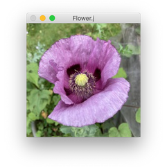


So insanely cool. Here is another nice image by David Kopacz with various autoPaletteSimplified versions.


And an image of some fruit. But this has a transparent background! How will OpenCV interpret that with no changes to our code? As a strange black background, apparently. Note that OpenCV does in fact support RGBA color values. That'd be a 4D Voronoi Diagram!


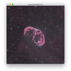
Lastly, let's do another awesome night sky photo, this one by Egil Sjøholt.


All very cool. Most of these photos started with between 30000-100000 distinct colors, so I think it's impressive that the color palettes with a few hundred colors are still nearly perfect!
And still so much to do! But we'll save that for next time.
Thank you for reading!
Jonathan M Gerhard


Comments